The Correction Panel¶

In the Correction panel, previously computed global corrections, such as from the Optics panel, can be visualised, reviewed and tested, with the goal to bring the measured machine as close as possible to nominal model conditions. It also gives access to the Knob Panel, which is used to turn a correction into a knob in the LSA database for use in operations. The panel is split into two sub-tabs: Correction and Correction test.

The default view is the Correction tab, which loads correction files and displays the powering change of the affected magnets or knobs from the selected correction. The Correction test tab will be covered further down, see checking corrections.

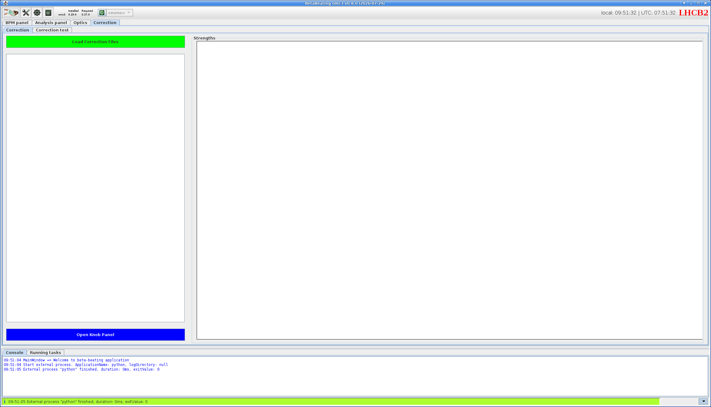
Correction Panel Default Look — The `Correction` panel's default appearance.

The Correction tab is organised into three areas. On the left is a table listing the loaded correction files, named as the relative path to the corresponding changeparameters_*.tfs file. Any correction computed in the Optics panel will appear here automatically. Clicking the Load Correction Files button above the table opens a dialogue to select and load previously determined corrections from disk.

To the right, the Strengths plot displays the powering change of each affected magnet or knob from the selected correction. Below the table, the Open Knob Panel button allows exporting a correction as a knob, see knob creation.

Recap: Correction Files

Each computed correction for a given parameter (e.g. phase) creates the following files in the Corrections folder:

A changeparameters_*.tfs file: the correction as a knob table, holding one powering delta per corrector — the change to apply to correct the machine (see viewing corrections).
A changeparameters_*_correct.madx file: the same correction (deltas) expressed as MAD-X assignments, to apply in order to correct the machine.
A changeparameters_*.madx file: the counterpart that instead makes the model reproduce the measurement; this is the file the correction test calls.
A changeparameters_*_gui.ini file: a record of the settings used for the run, written by the Python side process.

Viewing Corrections¶

Clicking an entry in the correction table on the left displays the corresponding powering changes in the Strengths plot on the right, with one bar per affected magnet or knob.

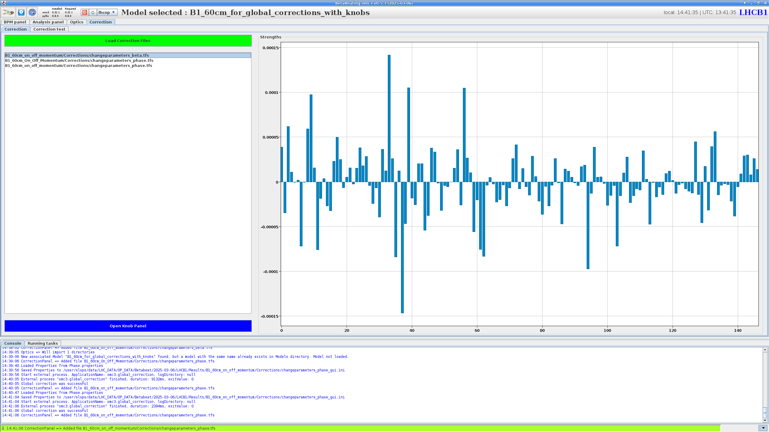
Correction Panel with Loaded Corrections and Strengths Plot — The `Correction` tab with correction files loaded; the `Strengths` plot on the right shows the powering change of each corrector for the selected correction.

These values are the change in powering of each element determined by the correction, a.k.a. the DELTA column of the corresponding changeparameters_*.tfs file. Hovering over a specific bar reveals the name of the magnet it corresponds to along with its exact value.

No Multi Selection

Note that unlike in the Optics panel, selecting multiple correction entries from the table will not lead to a comparison. This is due to the often different set of correctors modified by different corrections. Instead, only one of the corrections will have its strengths displayed.

The order of the plotted correctors is as given in the corresponding changeparameters_*.tfs file. As "correctors" in this case can be individual magnets, commonly powered magnet families or a specific set combined into a knob, the order might be arbitrary.

In the case of LHC corrections, the order is first by S location for known correctors, then alphabetically for unknown correctors. Check the get_variables() functions in the accelerator classes to figure out known correctors.

Global Coupling Corrections Trims

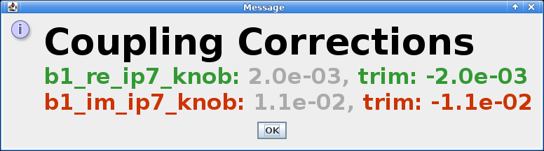
In the special case of global coupling corrections computed with the coupling preset, and to facilitate the user's work, double clicking on the correction file name in the table will spawn a popup detailing the exact trim to apply in the accelerator cockpit app.

Global coupling trim details — The global coupling trim popup, highlighting the exact determined corrections and corresponding trims to apply on each knob.

Checking Corrections¶

The Correction test tab lets one determine the effectiveness of a determined correction by showing its expected effect on the measurement's data. Running a correction then plots, for each correctable parameter, both the effect of the correction itself and the expected result of applying it.

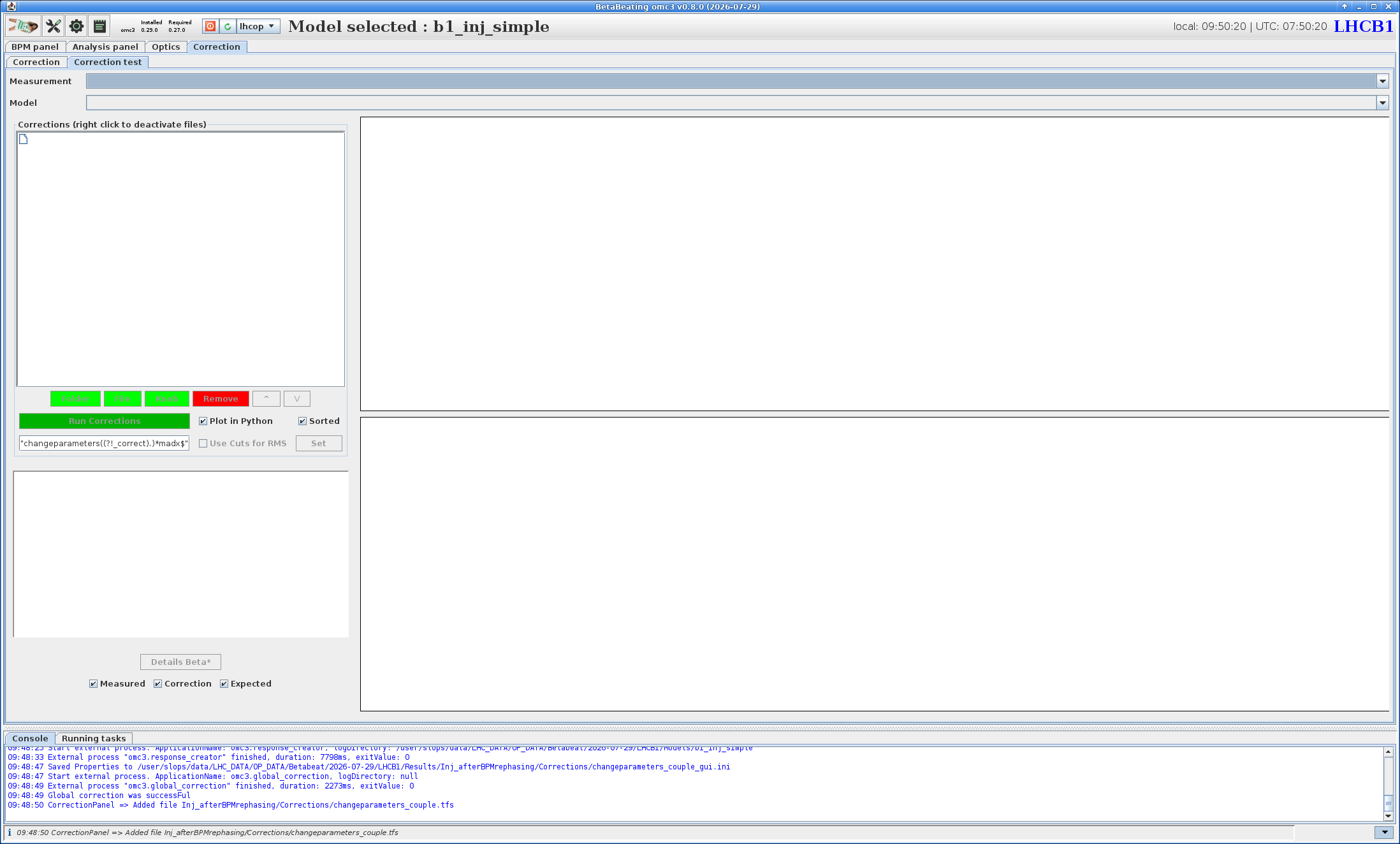
Correction Test Tab Default Look — The `Correction test` tab's default appearance.

Multiple corrections can be applied on top of one another (e.g. first a global correction followed by a local correction or an iteration) or in parallel, to be compared side by side.

Preparing a Test¶

One Measurement at a Time

The correction test only evaluates the effectiveness of one or more corrections on a single measurement at a time, and naturally the Correction test tab only allows managing corrections for one measurement at a time. To compare the impact of a correction on several measurements, you must run the indidivual correction tests manually on each.

At the top of the tab, two dropdown menus define the base data the correction test will use:

Measurement: the measurement to test. The dropdown lists entries known to the GUI (e.g. any measurement for which a correction was loaded in the previous tab), and an Other... entry that, when selected, opens a file dialogue to pick any measurement folder from disk.
Model: the model to apply the corrections to. It likewise lists known models (e.g. available in the Models menu) and also provides an Other... option with the behaviour stated above. Note that the model should naturally be one that matches the selected measurement.

The selected measurement then appears in the tree on the left, with its Corrections folder beneath it listing the available changeparameters_*.madx correction files.

Deactivating a Folder

Right-clicking a folder in the tree deactivates it, excluding it from the test correction run without removing it from the tree. This makes it easy to toggle a correction in or out of a comparative test run without having to delete and re-add it.

Different individual corrections can be tested and compared against one another. Different combinations of corrections can also be tested and compared against one another. The buttons below this table provide options to do so:

Folder: prompts for a name and creates a new corrections folder with that name. This button is always available, and the new folder is created as a sibling of the original Corrections folder in the tree (i.e. at the same level) within the selected measurement folder.
File: opens a file dialogue to pick a correction file — which should follow the changeparameters_*.madx naming and copies it into the selected folder. It is only available when a corrections folder is selected.
Knob: opens the Knob selection panel to search LSA for knobs, inspect their content, and import a chosen one as a file to include in the correction. Like File, it is only available when a corrections folder is selected.

Knob Import — Currently Not Working

The Knob button opens a Knob selection panel, but none of its controls currently have any effect.
Remove: removes the selected entry, file or folder, after a yes/no confirmation popup. Beware this button deletes the folder from disk, and a corrections folder can hold several files.

The correction test applies every file in it that matches the file filter, the regular expression shown at the bottom of the tab. By default this filter picks up the changeparameters_*.madx files output by the global correction process. It can be edited to select a different set.

Filter Field Known Issue

To pass the filter string correctly to Python, the expression string needs to be enclosed in double quotes. Most of the time Java does this automatically, but the quotes are sometimes lost after manual editing. As Java seems to be very inconsistent in this, a reliable fix has not been found yet. The best way to be sure is to check the Python command line printed in the log window after clicking Run Corrections and add the quotes manually if they are missing.

By combining the options above one can assemble several correction scenarios. The tabs below show a few typical setups of the corrections tree:

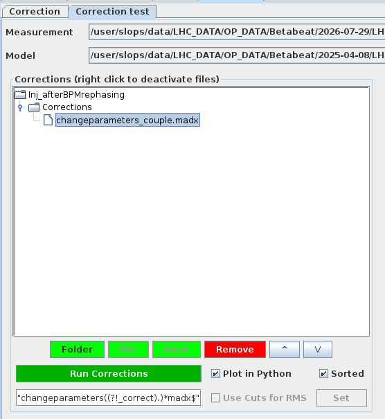
Single CorrectionCombined CorrectionComparing Schemes

Correction test tree with a single correction — A single correction in the `Corrections` folder: the test runs and plots just this one.

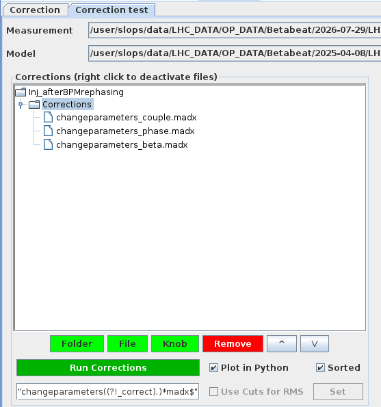
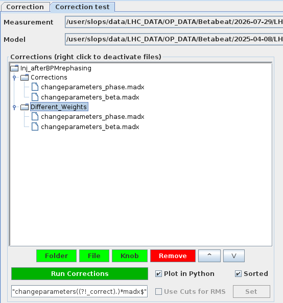
Correction test tree with several files in one folder — Several correction files placed in the same folder are applied *together* as one combined scheme.

Correction test tree with two correction folders — Two folders holding a similar correction, e.g. computed with different weights, to be compared.

Running the Test¶

Clicking Run Corrections then launches the test: each folder in the tree is run as a separate scenario, and the results are plotted together when done.

What Happens When Running a Correction

Under the hood, the GUI launches the omc3.check_corrections module, handing it the selected model and correction files, which:

Writes a job.create_twiss_matched.madx file in the Corrections folder, which calls the provided model and the correction files matching the filter,
Runs MAD-X to build the corrected ("matched") model,
Compares this matched model to the nominal one to determine the correction effect,
Uses data from the measurement to determine the expected result from applying this correction in the machine. This is done by subtracting the change between the nominal and matched models from the measurement data.

Two checkboxes next to the Run Corrections button control how the run behaves and where its plots go:

Plot in Python: should always be left ticked (its default) as the Java-side plotting has been removed. When checked, a Qt-based window opened by the Python process will display the results. If unchecked the run will still be performed and results saved to disk, but not interactive plot window will open.
Sorted: if checked (the default), the per-correction plot files are saved into their correction subfolders; otherwise they all go into the measurement directory.

Reading the Results¶

If Python plotting was enabled (which it is by default), a Correction Check window opens once the run finishes. It carries two sets of tabs:

Vertical tabs left of the window allow selecting one of the tested corrections.
Horizontal tabs are the top allow selecting the optics quantity to display (beta amplitude, beta phase, dispersion, f1001, f1010, orbit, phase, total phase)

The first left-hand tab is always All Corrections, and is a comparison overview. For the selected quantity it shows the Measurement values together with the expected end result of each tested correction, labelled by its folder name. As all curves are plotted as a deviation from the nominal model, a good correction is one that trends towards zero.

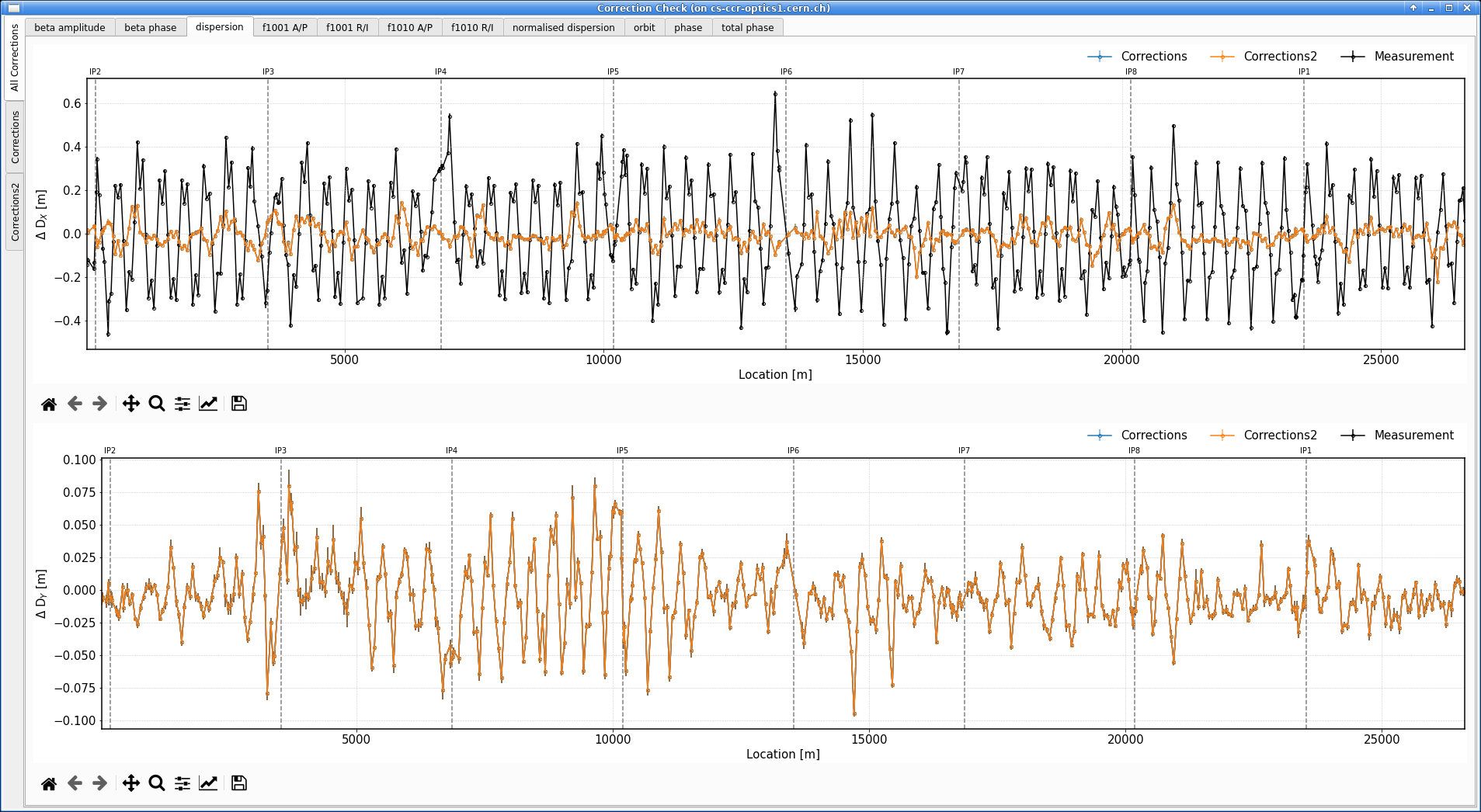
All Corrections results tab comparing schemes against the measurement — The `All Corrections` tab compares the expected end result of every tested correction against the measurement, here on the dispersion.

Each of the remaining left-hand tabs corresponds to one correction scheme (one folder from the tree). For the selected quantity it shows three curves:

Measurement: the measured deviation from the model.
Correction: the effect of the correction on the model, which aims to reproduce the measurement. A good correction lies on top of the Measurement curve.
Expected: the residual that would remain if the correction were applied to the machine. A good correction brings this close to zero.

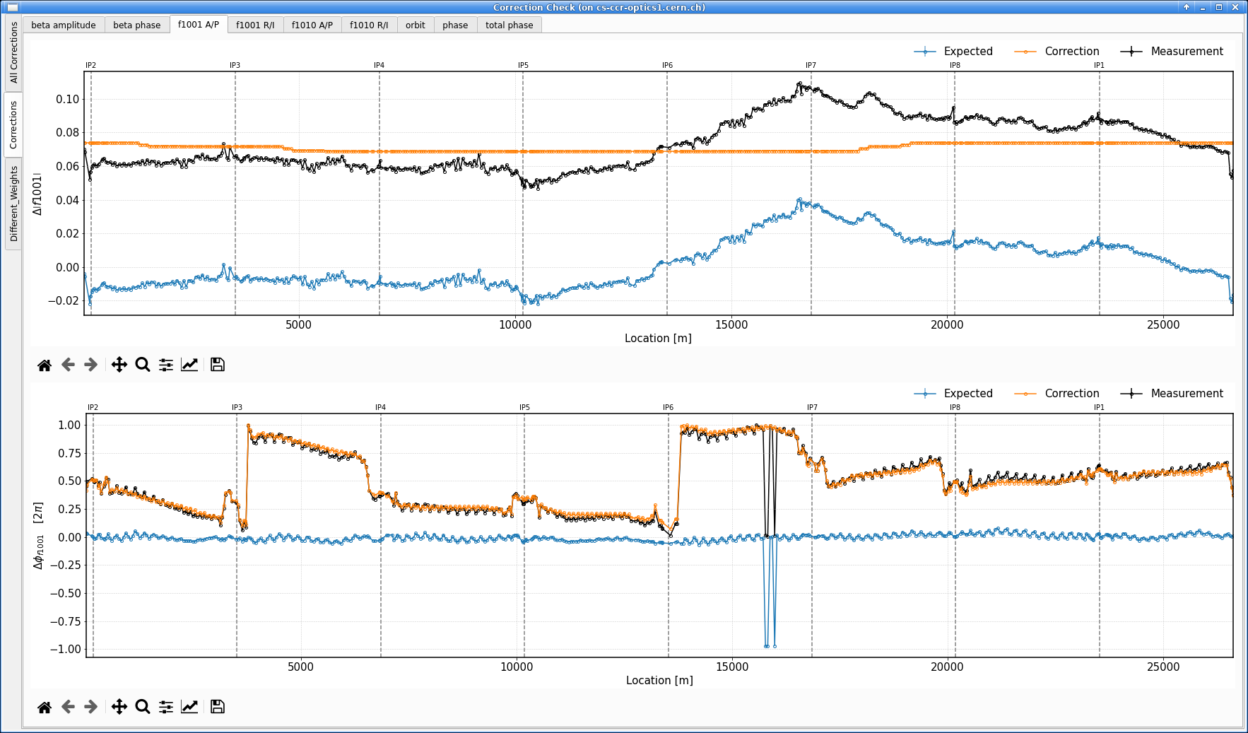
Per-scheme correction check results for a single scheme — A per-scheme view, showing the `Measurement`, the `Correction`, and the `Expected` residual, here on the `f1001` amplitude and phase.

Legacy Plotting Controls

The controls in the lower-left corner of the tab (the Details Beta* button as well as the Measured, Correction and Expected checkboxes) are remnants of the old Java-side plotting, which has been removed. They no longer have any effect and can be ignored.

Knob Creation¶

Once a correction has been validated with the correction test, it can be turned into a knob in the LSA database, ready to be trimmed into the machine during operation. This is done through the Knob Panel: back in the Correction tab, select the chosen correction in the table and click the Open Knob Panel button below it.

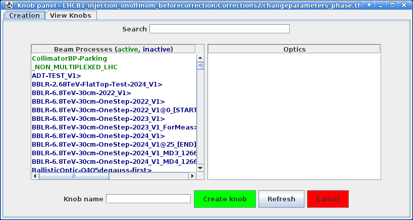
Knob Panel Creation tab default look — The `Knob Panel` on its `Creation` tab, opened for a selected correction.

Technical Network and Elevated Rights Needed

The Knob Panel communicates with LSA and therefore requires being inside the CERN Technical Network.

Furthermore, creating (and later deleting) a knob in LSA requires elevated rights, available through an EIC or the LHCOP account. Make sure a valid RBAC token has been acquired beforehand, via the log-in button at the top of the GUI.

Creating a Knob¶

A knob is created from the Creation tab, which opens by default, for the correction selected before opening the panel. The workflow is as follows:

Locate the target beam process in the Beam Processes list on the left and select it. At the top of the tab, a Search field helps filter the list.

Finding the Current Beam Process

The beam process currently used in the machine, a.k.a. active, is shown in green. The others are displayed in blue. This makes the relevant BP quicker to find.
With a beam process selected, the optics defined for it populate the Optics table on the right. Select every optic the knob should be defined for (use Ctrl+Left Button to add or remove entries to the selection, Shift+Left Button to select a range).
Enter a Knob name at the bottom.
Click Create knob to send its definition to LSA. Please follow the agreed upon naming conventions. If unsure, check previously created knobs and ask a senior team member.

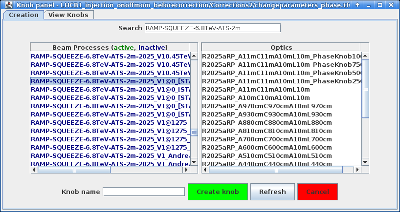
Selecting a beam processSelecting optics and naming the knob

Knob Panel with a beam process searched and selected, optics populated — A beam process filtered via `Search` and selected; its available optics now populate the `Optics` table on the right.

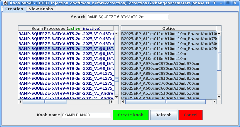
Knob Panel with optics selected and a knob name entered — The optics selected and a `Knob name` entered, ready to create the knob.

The Refresh button re-queries LSA to update the displayed lists, including the beam processes here and the knobs in the View Knobs tab; while Cancel closes the panel.

Viewing and Managing Knobs¶

The View Knobs tab lists the BETA-BEATING knobs created by the OMC team, again filterable through a Search field at the top. Selecting a knob displays its components (in LSA terms, a.k.a. powering circuits) either as a Table (components and their powering change) or as a Chart (like the Strengths plot in the Correction tab).

Table ViewChart View

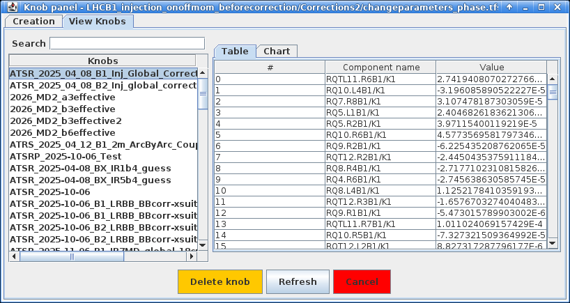
View Knobs tab showing a knob's components as a table — The `Table` view lists each component of the selected knob with its value.

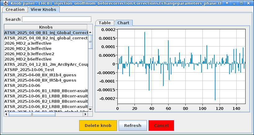
View Knobs tab showing a knob's components as a bar chart — The `Chart` view shows the same components as a bar plot, like the `Strengths` plot.

Note that a knob is only displayed here if a beam process and at least one optics are selected on the Creation tab.

Deleting Knobs

This tab provides a Delete knob button which will send a command to remove the selected knob from LSA. Use it with care! The effect is immediate.

What to do Now?

Your correction knob is defined and should already be available in LSA. It is time to trim it in the machine (ask the EIC on shift) and perform new measurements. Compare the corrected optics to the ones used to determine the correction to assess its effectiveness.