Amplitude Detuning Measurements
Note
Please keep in mind the general checks for measurements.
The Procedure in Short
The basis of this measurement is to kick with increasing amplitude in a single plane and perform fits over the resulting tune shifts. To assure a good direct and cross detuning measurement, it is important to check that both natural tune lines (for the horizontal and vertical tune) are visible in the respective spectrum. It is of utmost importance for the detuning analysis to perform rigorous cleaning on the data.
Measurement
Preparations
-
Confirm machine state
Make sure that the configuration of the machine is as you expect it.
- Perform the general checks
- Check correct \(\beta^*\)
- Check correct crossing angles
-
Check collimation sequence
"LOAD COARSE SETTINGS FOR NLO AT 30 CM" is the current (run 3, 2022) collimation sequence for AC-Dipole kicks in the LHC at \(\beta^*\) = 30cm up to ±170μrad IP1-V/IP5-H crossing and ±150μrad IP1-H, −150μrad to +140μrad IP5-V separation.
-
Correct Coupling
As always, coupling should be well corrected to \(|C-| \approx 10^{-3}\). This can be easily achieved by performing diagonal kicks of intermediate strength, and get the correction values from the GUI.
Beware that the signs need to be switched for correction in the machine. -
Do initial measurement
Start with a low AC-Dipole amplitude in both planes (e.g. 5%−10%) and analyse the resulting data.
-
Check both Natural Tunes are visible
Perform a quick harmonic analysis on the resulting data and check the spectrum. Both natural tunes need to be visible in their respective plane for the majority of BPMs. If not, maybe try to adapt the tune delta and move the driven tunes closer to the natural ones. See Info-box "Tune Deltas" below.
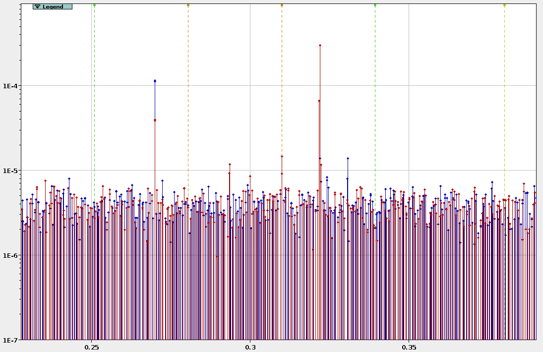
Bad Spectrum. 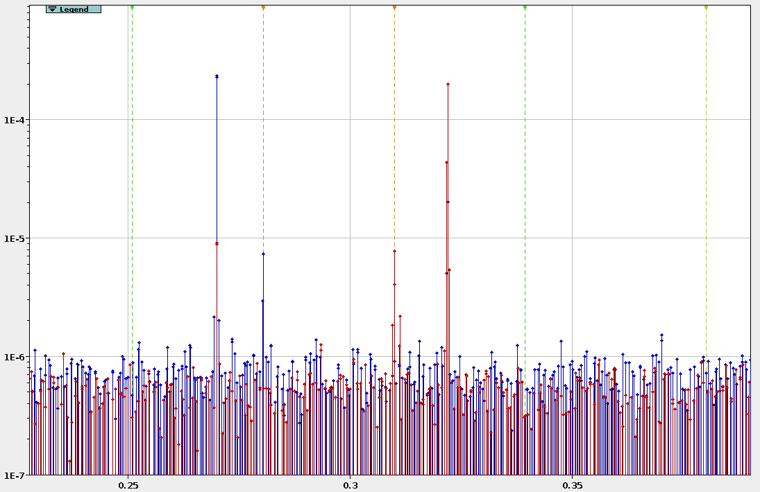
Good Spectrum. - Repeat until the spectrum looks usable
-
Tune Deltas
In the past, clean amplitude detuning measurements could be achieved with tune deltas (signs as given in Multiturn) of
Horizontal: -0.009,
Vertical: +0.007.
Actual Measurement
When kicking with crossing angles
When kicking with the crossing orbit bump in, make sure at each kick, that the losses occur in IP6/IP7 and not in the IPs with the crossing in (usually IP1 and IP5)! Losses in these IPs can appear with minor amplitude change, so keep the amplitude increase between kicks small. If you see losses in the IPs with crossing angles, but you are not yet happy with your maximum amplitude and you still have a lot of beam intensity left, you can kick at the same amplitude a few times and hope that the losses go down (the outermost particles are scraped) and then (carefully) continue increasing amplitude again.
-
Kicks in the vertical plane
While keeping the AC-Dipole amplitude in the horizontal plane constant (but not zero, to avoid weird AC-Dipole behaviour and to see if there is coupling effects), slowly increase the amplitude in the vertical plane.
- Kick with slowly increasing amplitude (1% - 5% increase between kicks)
-
Check losses are low during each kick
Adapt amplitude increase accordingly, as you do not want to dump the beam because the losses were to high. Also check the beam intensity, you will want to have good intensity if there are more detuning measurements in the other planes/settings to do. When kicking with crossing: head the warning above! Losses may occur with only a small amplitude increase!
-
Check for tune drift
If you are kicking with reduced tune deltas, it is also important to have an eye on the tune drift of the machine, so that you do not further decrease the distance between natural tune and excitation. Update the tune in Multiturn if necessary. The tune drifts will be compensated in the python analysis step by using data from the BBQ.
- Try to reach 0.015μm - 0.020μm in action (\(2J_x\))
- Get around 15 - 20 kicks
-
Kicks in the horizontal plane
While keeping the AC-Dipole amplitude in the vertical plane constant (but not zero, to avoid weird AC-Dipole behaviour and to see if there is coupling effects), slowly increase the amplitude in the horizontal plane.
- Kick with slowly increasing amplitude (1% - 5% increase between kicks)
-
Check losses are low during each kick
Adapt amplitude increase accordingly, as you do not want to dump the beam because the losses were to high. Also check the beam intensity, you will want to have good intensity if there are more detuning measurements in the other planes/settings to do. When kicking with crossing: head the warning above! Losses may occur with only a small amplitude increase!
-
Check for tune drift
If you are kicking with reduced tune deltas, it is also important to have an eye on the tune drift of the machine, so that you do not further decrease the distance between natural tune and excitation. Update the tune in multiturn if necessary. The tune drifts will be compensated in the python analysis step by using data from the BBQ.
- Try to reach 0.015μm - 0.020μm in action (\(2J_y\))
- Get around 15 - 20 kicks
-
Diagonal Kicks (optional)
To increase the accuracy of the cross-term measurement, 2D kicks (and 3.5D fitting) can be performed. If this is desired, it makes sense to throw some diagonal kicks, i.e. kicks with (more or less, not too important for the fitting) equal amplitude into the mix.
- Kick with slowly increasing amplitude (1% - 5% increase between kicks)
-
Check losses are low during each kick
Adapt amplitude increase accordingly, as you do not want to dump the beam because the losses were to high. Also check the beam intensity, you will want to have good intensity if there are more detuning measurements in the other planes/settings to do. When kicking with crossing: head the warning above! Losses may occur with only a small amplitude increase!
-
Check for tune drift
If you are kicking with reduced tune deltas, it is also important to have an eye on the tune drift of the machine, so that you do not further decrease the distance between natural tune and excitation. Update the tune in Multiturn if necessary. The tune drifts will be compensated in the python analysis step by using data from the BBQ.
- Try to reach 0.015μm - 0.020μm in action in both planes
- Get around 15 - 20 kicks
Action Estimation
The action can be calculated if \(\beta\) and peak-to-peak is known for a specific BPM by \(2J = \frac{(0.5 \cdot pk2pk)^2}{\beta}\). Otherwise it can always be checked running optics analysis on a file and looking into the Optics → Action/Tune tab or the kick-file.
Analysis
The analysis described here is performed with the Beta-Beat GUI omc3-v0.1.1, python package omc3 v0.4.0.
Earlier versions can analyse detuning as well, but some of the functionality described here is missing or a bit buggy,
e.g. in these versions the 2D-detuning analysis was newly implemented, as well as the Auto Clean functionality,
and the BBQ correction uses the wrong variable names. It is therefore recommended to use these or newer versions.
The analysis of amplitude detuning data requires very accurate estimates of the natural tunes, which can be hard to find if they get lost in the BPM noise or when they are close to resonances in the spectrum. Multiple features have been implemented in python and GUI to ease the detuning analysis.
As the main steps follow the standard optics analysis, the entries described here are mostly hints and tricks on how to optimise the analysis and only need to be applied where necessary.
-
Load Data
Simply load the data in the BPM panel. Make sure you are loading the correct data and check the logbook for misfired kicks etc.
-
Run Spectral Analysis
A bad spectral analysis can be recovered by the steps mentioned in "Cleaning", but a good frequency spectrum and well found natural tunes will save you a lot of time later on.
-
Small
tolerance(≈10−3)The tune tolerance (found in the
Tune Settings) specifies in what region around the assumed natural tune (see next step, the region is \(f\) ± tolerance), the highest frequency line is chosen to be the natural tune. To not accidentally capture the main tune or other excited resonances close by, the tolerance should be kept low (≈10−3). In case of large detuning (e.g. 40 · 103 m−1 × 0.016m = 6.4 · 10−3) or change of the AC-Dipole frequency (e.g. to adapt for tune drifts), this could mean that the natural tune will not fall into this window anymore. Both can be avoided usingAutotunesand maybe adapting the tune deltas (see next step), but can also be easily remedied in the cleaning step via theUpdate Nattunefunctionality. You can check the approximate tolerance window, by using theSet Windowbutton ofUpdate Nattune, which will set the markers according to theNattuneandtolerancein theTune Settings, which might differ a bit from the actual window ifAutotunesare used.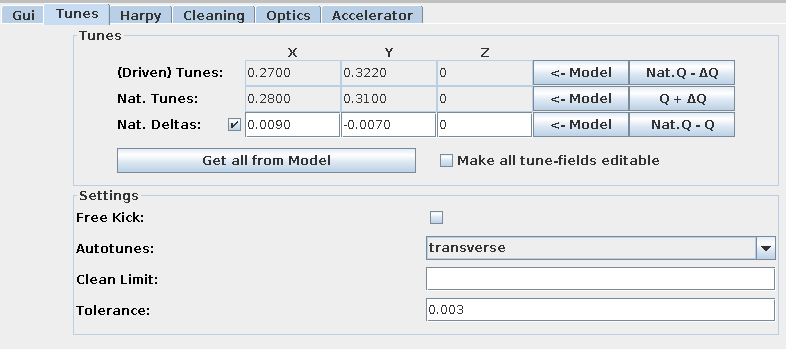
Tune settings. 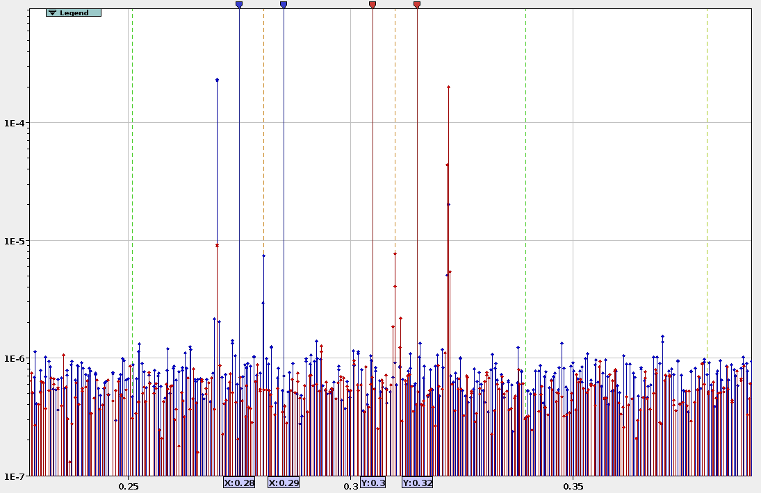
Approximate tolerance window, shown in blue for the horizontal and in red for the vertical tune. -
Use
AutotunesandNat. DeltasIn case the tunes do not coincide with the model, e.g. due to tune-drifts, we might run into problems when using a small tolerance (see previous step) as the natural tune might now be outside of the search window. One way to remedy that would be to also keep the model tunes up-to-date, e.g. use the exact tune values from the kick entries in the logbook. The one thing that should be constant during the measurement process though, are the tune deltas. The easiest way therefore, to make sure that at least the non-detuned tune is in the tolerance window, is to use the
Autotunesin theTune Settings: If this is activated (here fortransverseplanes), the highest peak in the whole spectrum is automatically assumed to be the driven tune. From those we can specify the difference to the natural tunes, by activating theNat. Deltas, instead of the natural tunes themselves. Now, no matter the tune drift (if the tunes are kept updated in Multiturn), the unperturbed natural tune should always be, where we expect it.
Beware that the signs between theNat. Deltasand Multiturn are inverted,
as Multiturn uses the Δ to specify the excitation frequency based on the natural tune, while the GUI/harpy searches for the natural tune at Δ from the driven tune.
Tune settings. -
Good Frequency Resolution (
TurnBits > 15)As the tune shift can be very small, we would want a good resolution in frequency, which can be controlled by
TurnBits. The standard value ofTurnBitsof20(leading to 220 complex coefficients, i.e. 221 spectral lines) is a good start, but can lead to excessive memory use when analysing 15−20 files at once. I estimate (from experience), that with19turn-bits, you will need 60GB to 80GB of RAM,20will obviously double and18halve that value. Both of these should be good values to use (see Infobox "TurnBit Estimation" below).
TheOutputBitson the other hand can be smaller, as the highest line stored per "bucket" will keep the frequency location calculated from the higher resolution formTurnBits. Therefore, even if the wrong line is selected (see step "Small tolerance"), the correct tune line will still be available in its bucket. The only issue would be, if there is a resonance really close by. A value of10-12(0.5 · 10−4 - 10−4 tune units) should be enough, to keep the file-size manageable and allow to open all the files simultaneously in the GUI.
-
-
Check and Clean Data
As mentioned before, it is of utmost importance to have clean data for the analysis as otherwise the fit will not work and yield unreasonable results. In principle each file needs to be checked that all BPMs point to the correct horizontal and vertical natural tunes, and cleaned appropriately. The following steps can be applied to recover the right natural tunes, if visible in the spectrum, limit error-bars and clean outliers.
-
Check Time and Space for
NATTUNEXandNATTUNEYFor the amplitude detuning analysis, the most important factor is the correct determination of the natural tunes. When the
harpyfrequency analysis is done, one can check the found tunes in theAnalysis Panelin theTime and Spacetab. Make sure to selectNATTUNEXandNATTUNEYnot just the main tunes.
Be sure that the found tune shown is the natural tune and not the driven tune.
Often it is required to check only one of them at a time, to get a clearer view. This can be easily achieved by right clicking into the data selection box on the left hand side of the plane that you want to unselect (or choosingnone) and then middle clicking into the chart to auto-zoom the data. The BPMs should differ only very little in the found tune (< 10−5), otherwise they need to be cleaned. The following steps describe how to do that.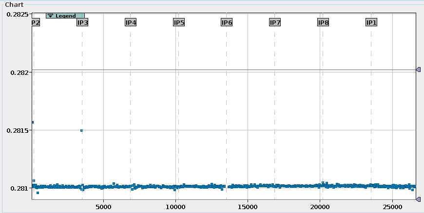
Example of NATTUNEXdata with outliers.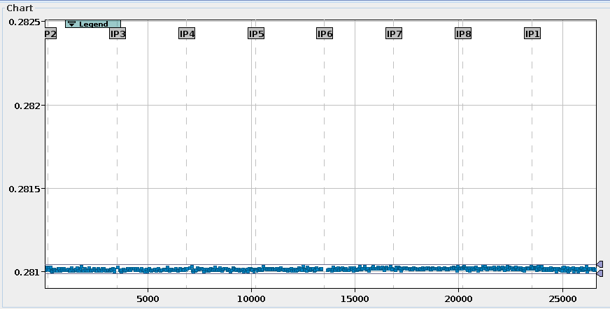
Example for clean (but not perfect) NATTUNEXdata. -
Check Frequency Chart
In case of differences in the found tunes of the BPMs, the first check should always be the
Frequency Chartin the adjacent tab of theAnalysis Panel. Especially, if there are clusters of found frequencies (i.e half of the BPMs agree on one frequency, the other half on another) in theTime and Space Chart, this hints at resonance lines close by that are mistaken for the natural tune. In any case, one needs to manually identify which of the lines within the selectedtolerance(see in one of the analysis steps above) is the actual tune. If it is not clear at first glance, compare the spectrum of the current kick with previous kicks to see the natural tune evolution with increasing amplitude. Once the right tune is identified - or determined of being not present in the spectrum - one of the next steps can be applied. Very helpful when trying to identify where the currently found natural tune is located in theFrequency Spectrum, is to activate theResonance Linesand selectNat. Tune (Measured), which shows the average natural tunes of all BPMs (of the first selected analysis data).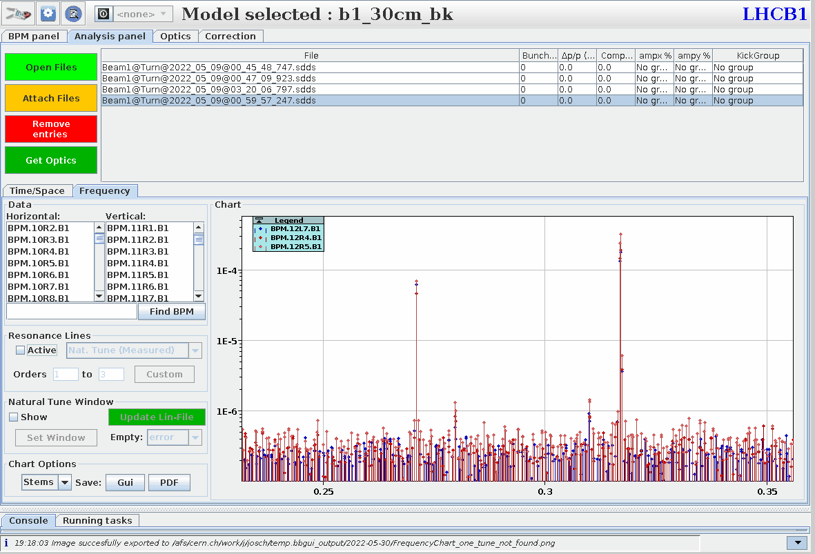
Show the natural tune in the frequency spectrum. -
Update natural tune window (where applicable)
If the correct natural tune is visible in the spectrum but could not be identified properly, due to resonance lines close by or because the line lies outside of the
tolerancewindow, one does not have to repeat the analysis with adapted tunes, deltas and tolerance window, as needs to be done when using the python2 GUI, but can use theUpdate Lin-Filefunctionality:- Select the BPMs you want to update.
If you want to update only one plane deselect (right click into the data selection box or choose
none) all BPMs in the other plane. If you want to update all BPMs in one plane, useCtrl + ain the data of the plane you want to select. (Minimize the legend first...)
ONLY SELECTED BPMS WILL BE UPDATED - Activate the
Natural Tune Windowby checkingshow. - Click
Set Windowif the vertical markers are not showing. - Set the markers so that the highest line they contain is the natural tune.
If there is no line for a selected BPM between the markers ( the window is
empty), it can either throw anerror,removethe bpm orignoreand leave the value as is.
(blue markers for the horizontal tune, red markers for the vertical tune). - Click
Update Lin-File.
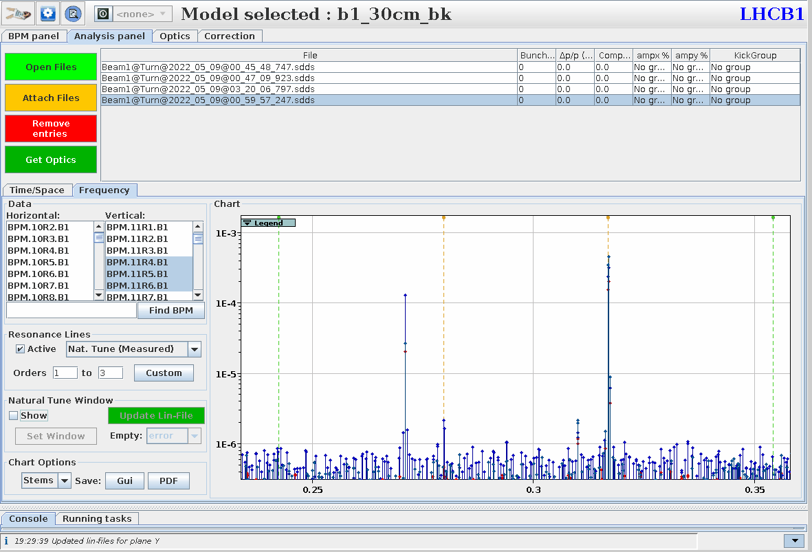
How to update the natural tune in the Lin-File. - Select the BPMs you want to update.
If you want to update only one plane deselect (right click into the data selection box or choose
-
Clean wrong BPMs (where applicable)
If updating the natural tune window from the last step is not sufficient (e.g. if the tune line is hidden in noise), the respective BPMs should be removed. Data can be manually cleaned by using the
Cleanfunctionality: Set the cursors around the data that you want to keep andClean. Or one can use theAuto Cleanfunctionality, which removes all outliers based on a gaussian distribution of the points until all points either lie inside the givenlimitor no points are beyond an automatically determined (by the number of points) range. In both cases, the majority of the BPMs should already agree on the natural tune and any cleaning step can be undone, either separately inXandYor intbothplanes.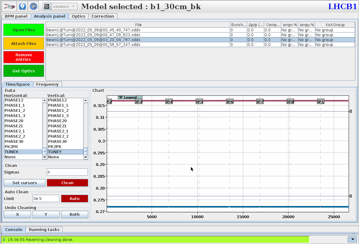
Auto CleanandUndoexample. -
Clean wrong Measurements (where applicable)
If the measurement is just very noisy and the natural tune can not be recovered using the
Update Lin-Fileor cleaning methods described above, it might be best to remove the measurement completely. If rigorous kicks have been performed, this might not be dramatic. In case one plane has resulted in a nice measurement, but the other not so much, this measurement might need to be manually cleaned in theKick Fileafter optics analysis, see in the later step.
-
-
Run combined Optics Analysis
After all measurements are satisfyingly cleaned, the optics analysis (
Get Optics) can be run on all measurements combined, so that they end up all in the same folder in the sameKick File(per plane). Give the analysis a nice name, identifying what kind of measurement you are doing (e.g.b1_ampdet_vertical_30cm_with_xing). -
Final Cleaning in Kick-Files
After the optics analysis has run, the only input from it that is needed for the detuning analysis are the
Kick-Files. In fact, these are the only files required to be present in the folder given as input to the pythonomc3.amplitude_detuning_analysisscript. In the case discussed above, that for one kick one wants to keep one tune plane but not the other, one can now open the respectivekick_xorkick_yfile and set the natural tune entry (e.g.NATTUNEX) for that kick toNaN. That way, this tune measurement will be ignored.
If you delete the whole line of the kick, you also remove the action data, which is needed to calculate the cross-term for this kick.
You would therefore also erase that datapoint, even though the measurement was fine. -
Run Amplitude Detuning Analysis
To run the amplitude detuning analysis, go in the
Optics Panelto theAction/Tune Taband select theopticsanalysis data. The GUI already allows for a quick check, if the data looks okay, e.g. no immensely large error-bars, outliers, etc. A quick and simple fit can already be performed here, with the slope being output in the logging line at the bottom. To start thepythonanalysis, clickPython Detuning Analysis. In theAmplitude Detuning Analysiswindow make sure that the rightAction Planefor your kicks is selected. ChooseXYfor the 2D/4D analysis. Also make sure, that the tick atAC-Dipoleis set, which will compensate the direct terms for the forced oscillations (i.e. divide the detuning by a factor of 2) in the plots. The analysis from the GUI is usually run with BBQ correction, which can bedeactivatedby choosing this option in theBBQ Filtering Method(it does not make sense to use the BBQ data without filtering first, therefore no filtering = no BBQ correction). Clicking onStartruns the amplitude detuningpythonscript on the current optics data and - if this is successful - also runs the plotting functions for the results (and the BBQ, if this function was not deactivated). This plotting is also done inpython, resulting inmatplotlibwindows to pop up andplot.ampdet_dQ*d2J*.pdffiles to appear in the optics result directory.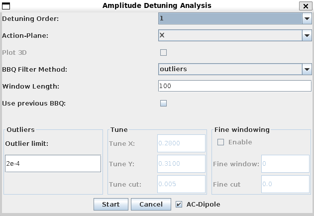
The amplitude detuning analysis window. -
With BBQ correction
To account for any tune drifts of the machine during the measurement, the tune data is corrected by the data from the BBQ. As this data is very noisy (and contains the outliers from the AC-Dipole excitation), it needs to be cleaned first. A moving average of the given
Window lengthis used determining a tune estimation over the kick timerange. This data is extracted from timber and saved into abbq_ampdet.tfsfile in the optics results folder. So in case you run the same detuning analysis again, but maybe want to modify the BBQ cleaning parameters, this data can be reused by tickingUse previous BBQ. The first cleaning methodoutliersis using the same algorithm asAuto Clean, and requires anoutlier limitto be set. BBQ data deviating less than this limit from the moving average are never cleaned. The moving average is then calculated on the cleaned data and the closest value to the kick time subtracted from the natural tune measured during the kick. The second methodcutallows to choose a fixedcutaround the assumed natural tunes and data beyond that value is cleaned. In this case alsoFine windowingcan be enabled, which performs another moving average on the now cleaned data and data-points deviating more than thefine cutvalue are also cleaned.
-
Quick TurnBit Estimation
Let's assume a small detuning of 10 · 103 m−1 and an action increase between kicks of 0.020 μm / 20 kicks,
leading to a detuning difference between two kicks of ΔQ = 1 · 10−5.
The frequency resolution \(\Delta f\) is the inverse of the length of the turns-data (halved, as we have pairs), so 2−TurnBits−1 :
TurnBits = 20: \(\Delta f = 4.8 \cdot 10^{-7}\)
TurnBits = 19: \(\Delta f = 9.5 \cdot 10^{-7}\)
TurnBits = 18: \(\Delta f = 1.9 \cdot 10^{-6}\)
TurnBits = 17: \(\Delta f = 3.8 \cdot 10^{-6}\)
TurnBits = 16: \(\Delta f = 7.6 \cdot 10^{-6}\)
TurnBits = 15: \(\Delta f = 1.5 \cdot 10^{-5}\)
We therefore need to set TurnBits to at least 16 to assure that we will see the change ΔQ between kicks.