Determining Corrections¶

After having identified potential sources of errors through the forward and backward propagation, the next step is to determine and test corrections. This page covers how to apply corrections in the GUI, test different correction schemes and interpret the resulting plots.

Run Matcher — Not Implemented

In the future, the Run Matcher button is intended to launch an automated matching routine for the currently selected optics and segment. This would calculate corrections and produce a correction file that can then be loaded in the corrections dialogue and further modified.

Applying Corrections¶

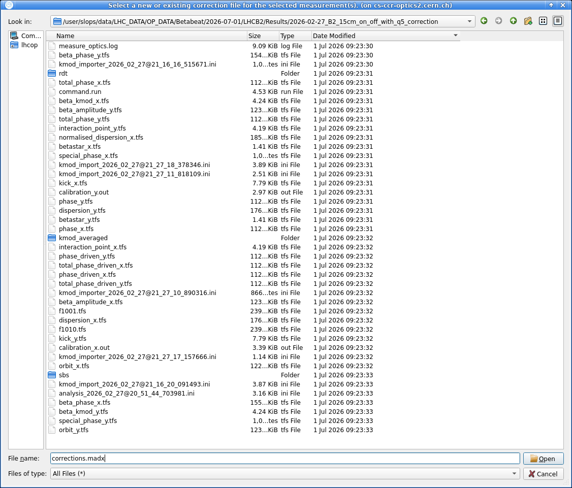
Clicking the Corrections button in the side panel opens the corrections dialogue, where you can load or create a correction file to apply to the model. To create a file, simply type a name (e.g. corrections.madx) in the File name field and press the Open button to the right. See the screenshot below.

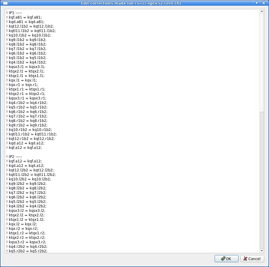
Correction File Dialog — The correction file dialogue, prompting to load or create a correction file. Creating a new file works by entering a name.

After creating or selecting a correction file, a new window displays its contents directly and allows you to edit it. If a correction file has already been associated, clicking the Corrections button will open the editor directly.

Corrector Suggestions

When a default correction file is created and default segments have been added, correctors may be suggested provided this feature is activated in the settings. The screenshot below shows the correction file editor with suggested correctors for the LHC's default segments.

Correction File Editor with Defaults — The correction file editor, here showing suggested correctors for LHC default segments.

Note that the correction file path is applied to all currently selected optics.

If some of the selected measurements already have the same correction file loaded while others do not, a dialogue will ask whether to apply the same correction file to all of them. If there is a conflict between different correction files across the selected optics, an error message will show.

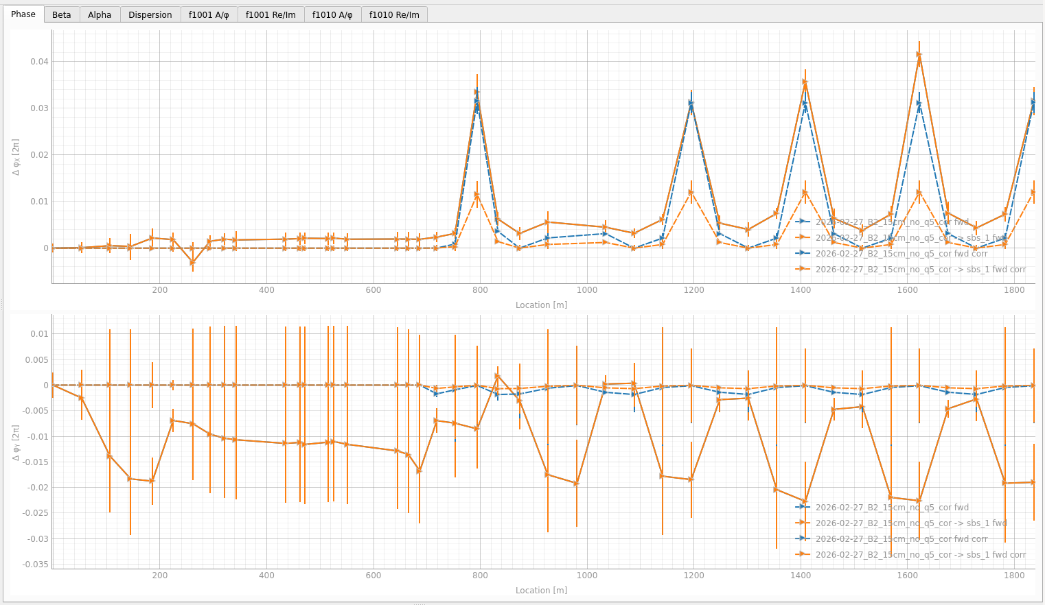
After editing the correction file, click OK then run the propagation again (with Run Segment(s)) to compute the effect of the attempted correction. After running the segment, the plots update to show the corrected results as dashed lines, in addition to the solid propagated measurement line. What these dashed lines represent depends on the plot settings, as detailed in Corrected and Expected Plots below.

Sign Conventions

The corrections applied in the GUI should modify the model to match the propagated measurement. In order to actually correct the machine, these corrections generally need to be inverted: they represent what error in the model would reproduce the observed measurement deviation, and the opposite of that error is what should be applied operationally. Be aware, however, that sign conventions may differ between MAD-X and LSA and care must be taken when translating correction values from the GUI to the control system.

In practice for the LHC IRs, using MQX?->K1 element strengths to reproduce errors requires a sign change when converting to LSA, for all triplets. However, the ktqx2 knob (used in MAD-X) already carries a sign opposite to LSA Q2 (unlike ktqx1 or kqx), so its LSA conversion cancels out: no sign change (or rather a double sign change) is needed.

Corrected and Expected Plots¶

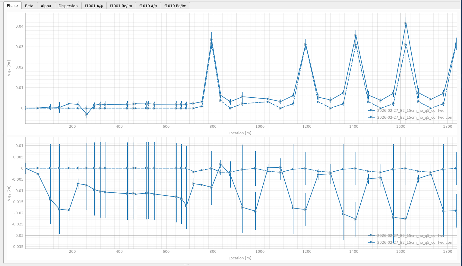
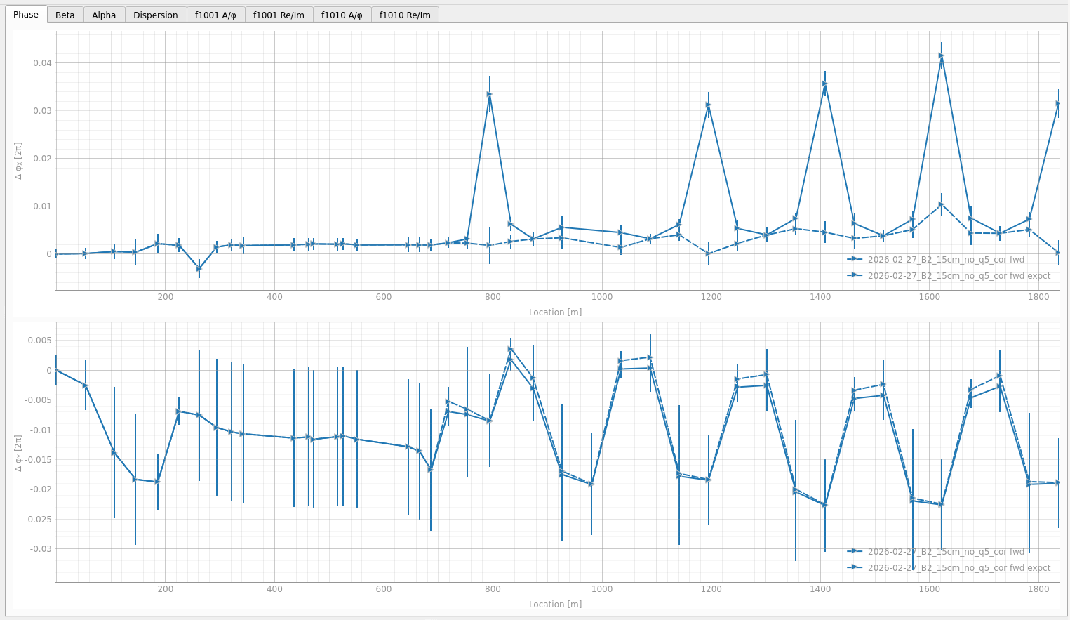
The plot settings let you choose what the dashed line represents:

Matched value (corr): the difference between the propagated corrected model and the nominal propagated model. If the correction successfully reproduces the measured errors, this dashed line should lie close to the solid propagated measurement line.
Expected value (expct): the difference between the measured values and the propagated corrected model. This represents the expected outcome after the correction has been applied to the machine, and should therefore be close to zero for the correction to be effective.

The tabs below illustrate each setting for the same correction:

Matched (corr setting)Expected (expct setting)

Matched Correction Effect (corr) — A good correction reproduces the effect observed in the machine, so the dashed line lies close to the solid propagated measurement.

Expected Correction Effect (expct) — A good correction compensates the observed deviation, so the dashed residual line lies close to zero.

Testing Multiple Correction Schemes¶

A practical approach to testing different correction strategies is to create virtual copies of the same measurement. To do so, click the Copy button in the loaded optics section to create a virtual copy.

This copy references the same input measurement data but writes its output to a separate directory, making it possible to try multiple correction schemes side by side without duplicating files on disk. In the side panel, virtual copies are displayed as NAME -> OUTPUT_DIR_NAME to distinguish them from the original optics entry.

Two Correction Schemes Compared on the Phase — Comparing two correction schemes on the phase, using virtual copies of the same measurement — the dashed blue correction outperforms the dashed orange one.

Similarly, creating multiple segments with different start BPMs for the same region lets you evaluate sensitivity to the starting point. This helps confirm whether the correction holds regardless of which BPM anchors the propagation.