Loading Data and Running Segments¶

The first step in a segment-by-segment analysis is loading data and running a segment to propagate the measured properties through the machine's model. This page showcases the interface and workflow to do so.

Loading Measurement Data¶

If started from the Beta-Beat GUI with an optics analysis selected, the corresponding optics data and associated model will be automatically loaded.

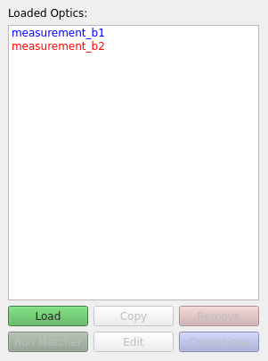
To load (additional) measurements, click the Load button in the side panel to open a file dialogue and select the measurement folder corresponding to the optics analysis to be loaded.

It is possible to directly point to an existing SbS output folder, which is useful when resuming previous work or when a different output directory name than the default sbs was used.

Once loaded, the optics entries will appear in the side panel, colour-coded by beam. Hovering over an optics name displays a tooltip with a summary of its associated paths and accelerator parameters.

The SbS analysis output is by default stored in a folder named sbs within the corresponding optics folder. If the corresponding option is activated in the settings, the GUI will automatically scan the sbs folder for existing segment results and load them into the segments table when loading the data.

Editing Optics

The edit dialogue can be opened by clicking the Edit button or by double-clicking the optics name in the side panel. It allows one to modify the paths and accelerator parameters associated with the loaded optics.

Note that the measurement path itself cannot be changed from this dialogue. To use a different measurement directory, load a new measurement folder instead.

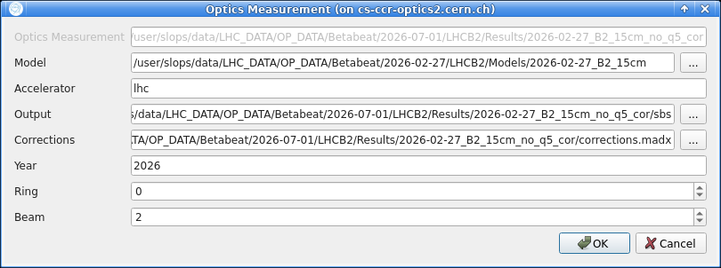
The available fields are:

• Model: Path to the model folder, which should contain the optics files for the model.
• Accelerator: Accelerator name, e.g. lhc, sps, ps, psbooster.
• Output: Path to the output folder where the SbS analysis results are stored. Defaults to sbs within the measurement folder.
• Corrections: Path to the correction file containing all corrections to be applied to the model. The corrections are executed by MAD-X as-is to correct the model, so they must be written in MAD-X syntax and represent the "inverse" of the corrections applied in the machine (MAD-X/LSA sign conventions apply). See determining corrections.
• Year: Year of the accelerator optics to use, corresponding to the acc-models branch from which the appropriate model is created. See the omc3 model creation.
• Ring: Ring to use, if applicable (relevant for PSB).
• Beam: LHC beam to use, if applicable, e.g. 1 or 2.

The parameters are validated when clicking OK. Which parameters are required depends on the selected accelerator.

To remove an optics entry from the GUI, select it and click the Remove button. This only unloads it from the interface and does not delete any files from disk.

Defining Segments¶

Before running any propagation it is necessary to define segments. Each segment is defined by a name, a start element and an end element. Segments can be added by first selecting a loaded optics measurement.

Default Segments¶

The quickest way to get started is to click the Add Defaults button, which populates a predefined set of segments appropriate for the currently selected accelerator.

For instance, in the LHC the default segments cover IP1, IP2, IP5 and IP8. Each spans from BPM.L12 to BPM.R12 and contains one of the main interaction points. They are therefore of particular interest for the LHC analysis.

Custom Segments¶

It is possible to create an arbitrary custom segment by clicking the New button. This opens the segment editor dialogue, as shown below.

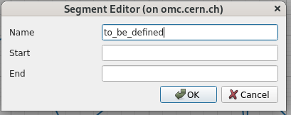
In the dialogue, enter the segment name along with the start element and end element. The SbS GUI will automatically find the closest BPMs before and after the named element to use as the propagation boundaries.

The Copy button here duplicates the currently selected segment under a new name, which is useful for quickly creating variants, for instance with different start BPMs, to evaluate how the choice of starting point affects the results. A separate Copy button in the loaded optics section instead duplicates an entire measurement, used when testing multiple correction schemes.

The Remove button deletes the selected segment from the table. This only removes the definition from the GUI and does not delete any output files from disk.

New segments will display in the segments table, as shown below.

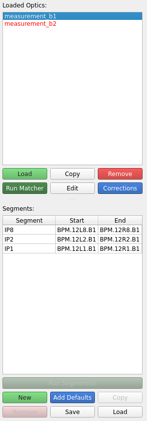
It is possible at any time to edit a given segment's properties by double clicking either the Segment, Start or End entry in the table and changing its content.

Running Segments¶

Once segments are defined, for a given optics select the segments to propagate measured properties through, then click the Run Segment(s) button.

The GUI calls MAD-X to propagate optics parameters from the start and end BPMs through each defined segment. The propagated values are then compared against the measured data and deviations are computed.

Measured errors are also propagated through the segment analytically, and added in quadrature to the measurement uncertainty.

While the propagation is running in the background, a spinner icon appears at the bottom right of the GUI. Hovering over the running tasks text next to the spinner displays the name of the currently running task (e.g. SbS for <optics name>).

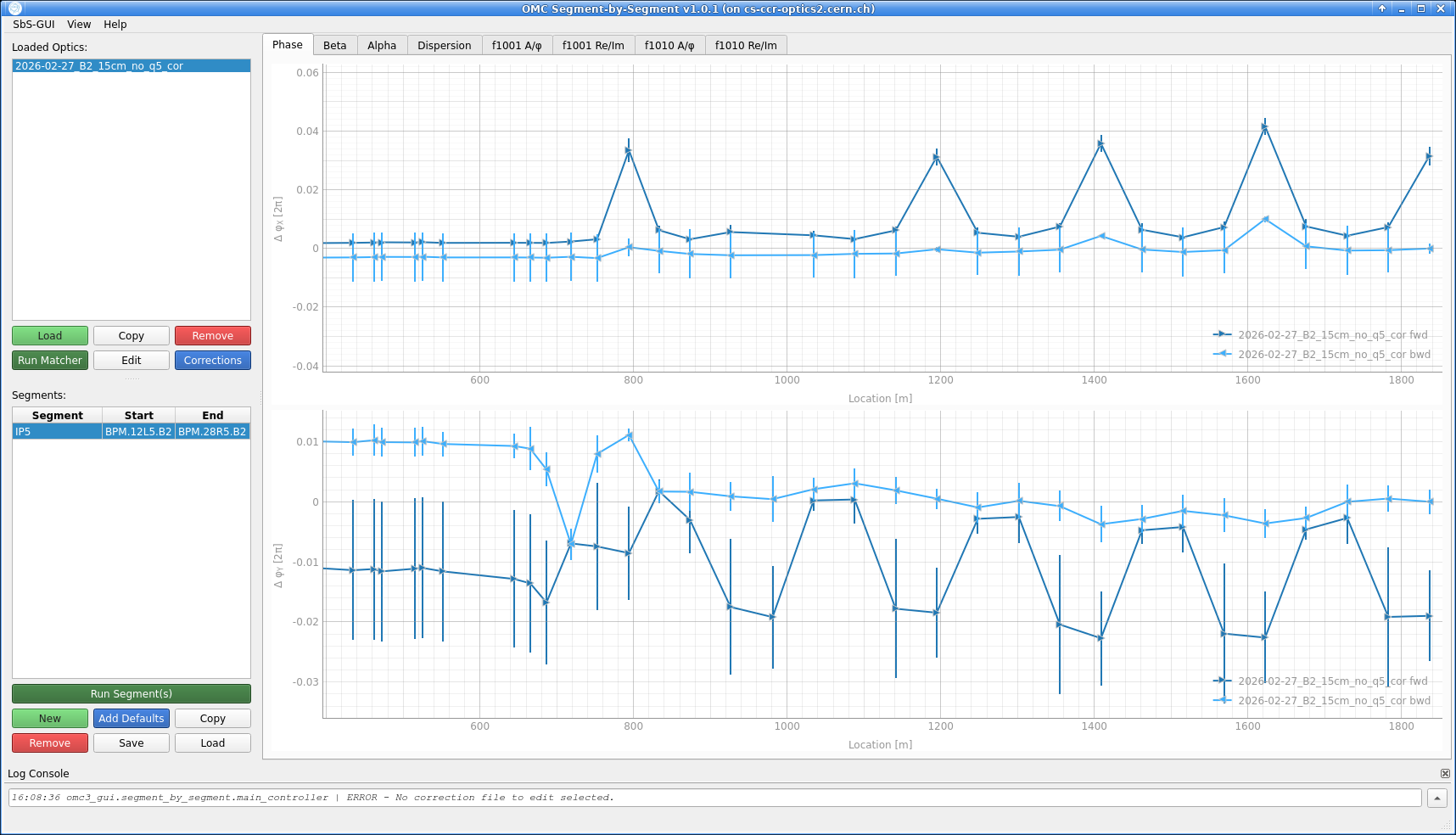
Inspecting Results¶

After the propagation has completed for a segment, selecting it in the segments table will display its results in the main plot area. By default the plot shows the difference between the propagated model and the measurement. This view allows one to identify where discrepancies exist and pinpoint the locations of optics errors.

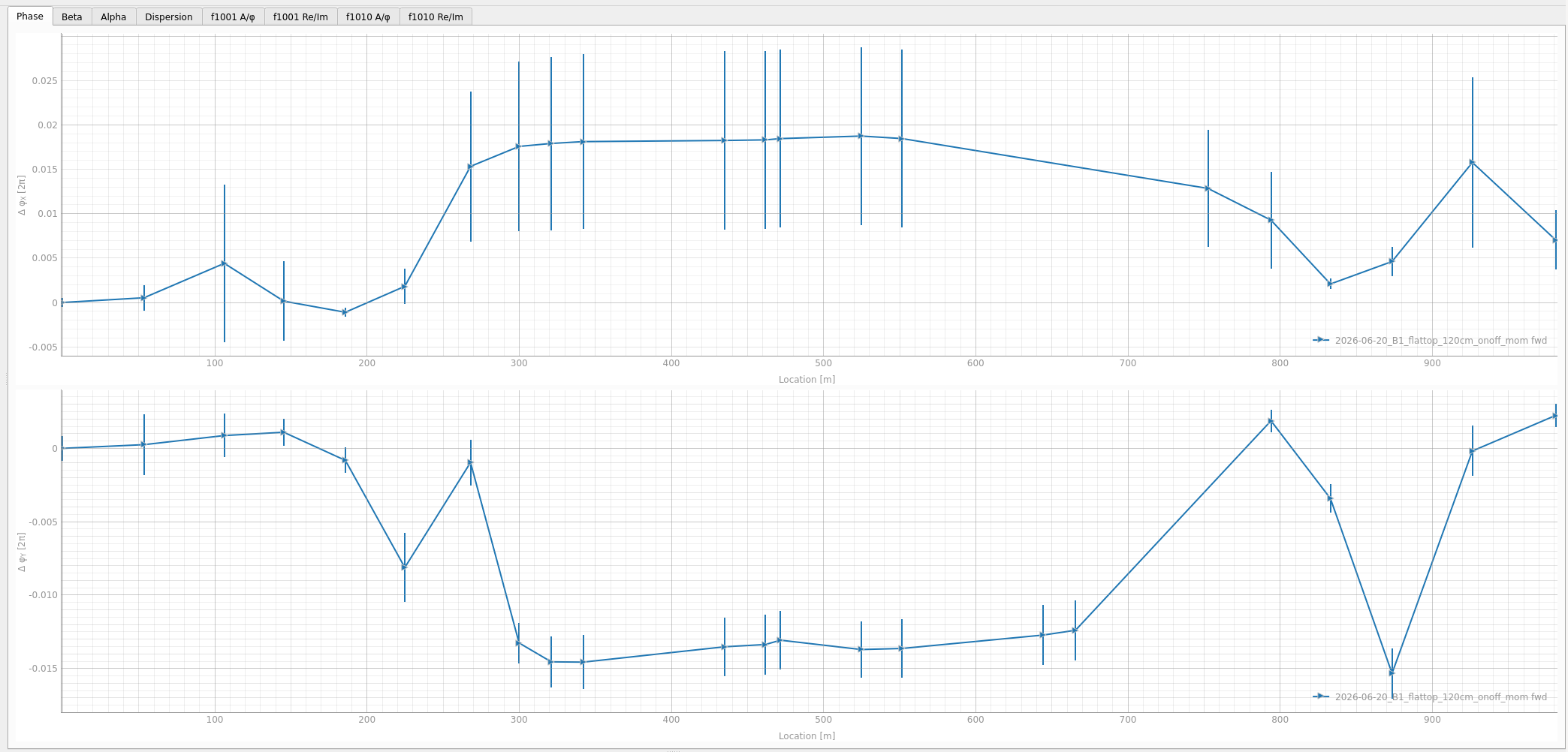
The solid line represents said difference under the assumption that the model and measurement share the same value at the start BPM (or end BPM for backward propagation). Arrow markers indicate the direction of the propagation: rightward arrows for forward propagation and leftward arrows for backward propagation.

Inspecting both directions helps confirm the error source: if deviations appear after the same location from both sides, that location is likely where the error originates. Below is such an example from the LHC 2026 commissioning: forward and backward propagation helped confirm the issue was located at the Q5.R5B2 quadrupole, located at around the 700m mark in the segment.

The tabs above the plot area allow switching between the different optics parameters propagated through the segments, such as the phase advance, the \(\beta\)-function or coupling RDTs.

Once optics errors have been identified, see determining corrections on the next page for how to test corrections.

Comparing Multiple Segments or Optics¶

When multiple optics are loaded simultaneously, identically defined segments (sharing the same name, start BPM and end BPM) are automatically grouped together and overlaid on the same plot when selected together.

This grouping makes it straightforward to compare results from different measurements or different correction schemes for the same segment of the accelerator. Hovering over a segment entry in the table displays a tooltip showing which loaded optics it belongs to and whether propagation has been run.

When multiple segments are selected, the default behaviour is to only plot together those that share the same start BPM, since the horizontal axis position is relative to the start of the segment.

This constraint can be relaxed via the Same segment start option in the plot settings, although doing so is generally not recommended as it can lead to confusion when comparing positions. Activating the Model Location option changes the horizontal axis to show absolute positions in the accelerator rather than positions relative to the segment start, which makes it meaningful to overlay segments with different start BPMs and compare their results directly.

Each combination of segment and optics is assigned a consistent colour, while different markers and line styles distinguish forward propagation, backward propagation, corrected and expected traces (see Determining Corrections for details on these). When plotting many segments at once, it is advised not to activate all trace types simultaneously, as the plot can become very crowded and difficult to read.